Video Scene Location Recognition Using AI: Experiments

Table of Links

Abstract and Introduction

ANN-Based Scene Classification

Methodology

Experiments

Conclusion and Future Research, Acknowledgments and References

4 Experiments

4.1 Experimental Setup

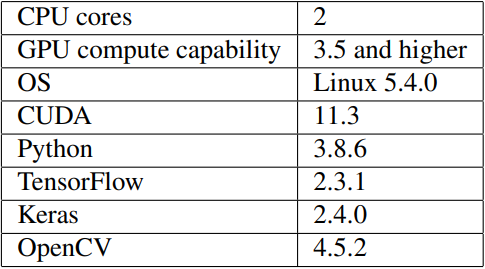
The ANNs for scene location classification were implemented in the libraries Python language using TensorFlow and Keras. Neural network training was accelerated using a NVIDIA GPU. The versions of the employed hardware and software are listed in Table 1. For image preparation, OpenCV and Numpy were used. The routine for preparing frames is a generator. It has lower capacity requirements, because data are loaded just in time when they are needed and memory is released after the data have been used for ANN. All non-image information about inputs (video location, scenes information, etc.) are processed in text format by Pandas.

We have 17 independent datasets prepared by ourselves from proprietary videos of the The Big Bang Theory series, thus the datasets can’t be public. Each dataset originates from one episode of the series. Each experiment was trained with one dataset, so results are independent as well. So we can compare behavior of the models with different datasets.

Our algorithm to select data in training routine is based on oversampling. It randomly selects target class and from the whole training dataset is randomly select source scene with replacement. This algorithm is applied due to an unbalanced proportion of different target classes. Thanks to this method, all targets are distributed equally and the network does not overfit a highly represented class.

4.2 Results

Summary statistics of the predictive accuracy of classification all 17 episode datasets are in Table 3. Every experiment was performed on every dataset at least 7 times. The table is complemented with results for individual episodes, depicted in box plots.

The model with a max-pooling layer had the worst results (Figure 12) of all experiments. Its overall mean accuracy was around 10 %. This is only slighty higher than random choice which is 1/12. The model was not able to achieve better accuracy than 20 %. Its results were stable and standard deviation was very low.

Slightly better results (Figure 10) had the model with the a flatten layer, it was sometimes able to achieve a high accuracy, but its standard deviation was very high. On the other hand, results for some other episodes were not better than those of the max-pooling model.

A better solution is the product model, whose predictive accuracy (Figure 9) was for several episodes higher than 80 %. On the other hand, other episodes had only slightly better results than the flatten model. And it had the highest standard deviation among all considered models.

The most stable results (Figure 11) with good accuracy had the model based on average-pooling layer. Its mean accuracy was 32 % and for no episode, the accuracy was substantially different.

The model with unidirectional LSTM layer had the second mean accuracy of considered our models (Figure 13). Its internal memory brings advantage in compare over the previous approaches, over 40 %, though also a comparatively high standard deviation.

The highest mean accuracy had the model with a bidirectional LSTM layer (Figure 14). It had a similar standard deviation as the one with a unidirectional LSTM, but an accuracy mean nearly 50 %.