Authors:
(1) Lukáš Korel, Faculty of Information Technology, Czech Technical University, Prague, Czech Republic;
(2) Petr Pulc, Faculty of Information Technology, Czech Technical University, Prague, Czech Republic;
(3) Jirí Tumpach, Faculty of Mathematics and Physics, Charles University, Prague, Czech Republic;
(4) Martin Holena, Institute of Computer Science, Academy of Sciences of the Czech Republic, Prague, Czech Republic.
Table of Links
ANN-Based Scene Classification
Conclusion and Future Research, Acknowledgments and References
3 Methodology
3.1 Data Preparation
Video data consists of large video files. Therefore, the first task of video data preparation consists in loading the data that is currently needed.
We have evaluated the distribution of the data used for ANN training. We have found there are some scenes with low occurence, whereas others occur up to 30 times more frequently compared to them. Hence, the second task of video data preparation is to increase the uniformity of their distribution, to prevent biasing the ANN to most frequent classes. This is achieved due to undersampling the frequent classes in the training data.
The input consists of video files and a text file. The video files are divided into independent episodes. The text
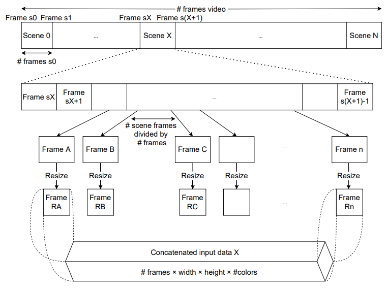
file is contains manually created metainformation about every scene. Every row contains metainformation about one scene. The scene is understand as sequence of frames, that are not interrupted by another frame with different scene location label. Every row contains a relative path to the source video file, the frame number where the scene begins and the count of the its frames. Figure 1 outlines how frames are extracted and prepared for an ANNs. For ANNs training, we select from each target scene a constant count 20 frames (denoted # frames in Figure 1). To get most informative representation of the considered scene, frames for sampling are taken from the whole length of the scene. This, in particular, prevents to select frames only within a short time interval. Each scene has its own frame distance computed from its frames count:
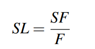
where SF is the count of scene frames, F is the considered constant count of selected frames and SL is the distance between two selected frames in the scene. After frames extraction, every frame is reshaped to an input 3D matrix for the ANN. Finally the reshaped frames are merged to one input matrix for the neural network.
3.2 Used Neural Networks and Their Design
Our first idea was to create a complex neural network based on different layers. However, there were too many parameters to train in view of the amount of data that we had. Therefore, we have decided to use transfer learning from some pretrained network.
Because our data are actually images, we considered only ANNs pretrained on image datasets in particular ResNet50 [9], ResNet101 [9] and VGGnet [2]. Finally, we have decided to use VGGnet due to its small size.
Hence, ANNs which we trained on our data are composed of two parts. The first part, depicted in Figure 2 is based on the VGGnet. At the input, we have 20 frames
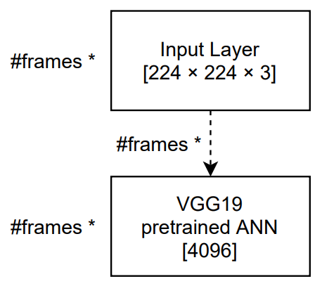
(resolution 224×224, BGR colors) from one scene. This is processed by a pretrained VGG19 neural network without two top layers. The two top layers were removed due to transfer learning. Its output is a vector with size 4096. For the 20 input frames we have 20 vectors with size 4096. These vectors are merged to a 2D matrix with size 20×4096.
For the second part, forming the upper layers of the final network, we have considered six possibilities: a product layer, a flatten layer, an average pooling layer, a max pooling layer, an LSTM layer and a bidirectional LSTM layer. All of them, as well as the VCGnet, will be described below. Each of listed layers is preceded by a Dense layer. The Dense layer returns matrix 20×12, where number 12 is equal to the number of classes. With this output every model works differently.
VGGnet The VGGNets [2] were originally developed for object recognition and detection. They have deep convolutional architectures with smaller sizes of convolutional kernel (3×3), stride (1×1), and pooling window (2×2). There are different network structures, ranging from 11 layers to 19 layers. The model capability is increased when the network is deeper, but imposing a heavier computational cost.
We have used the VGG19 model (VGG network with 19 layers) from the Keras library in our case. This model [3] won the 1st and 2nd place in the 2014 ImageNet Large Scale Visual Recognition Challenge in the 2 categories called object localization and image classification, respectively. It achieves 92.7% in image classification on Caltech-101, top-5 test accuracy on ImageNet dataset which contains 14 million images belonging to 1000 classes. The architecture of the VGG19 model is depicted in figure 3.
3.2.1 Product array
In this approach, we apply a product array layer to all output vectors from the dense layer. A Product array layer
![Figure 3: Architecture of the used VGG19 model [10], in our network is used without FC1, FC2 and Softmax layers](https://cdn.hackernoon.com/images/fWZa4tUiBGemnqQfBGgCPf9594N2-n4b3zk9.png)
computes product of all values in chosen dimension of an n-dimensional array and returns an n-1-dimensional array.
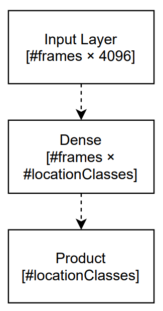
A model with a product layer is outlined in Figure 4. The output from a Product layer is one number for each class, i.e. scene location, so our result is vector with 12 numbers. It returns a probability distribution over the set of scene locations.
3.2.2 Flatten
In this approach, we apply a flatten layer to all output vectors from the dense layer. A Flatten layer creates one long vector from matrix so, that all rows are in sequence.
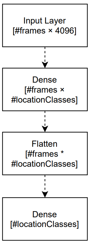
A model with a flatten layer is outlined in Figure 5. After the input and a dense layer, a flatten layer follows, which returns long vector with 12 ∗ 20 numbers in this case. It is followed by a second dense layer. Its output has again a dimension equal to the number of classes and it returns a probability distribution over the set of scene locations.
3.2.3 Average Pooling
In this approach, we apply average pooling to all output vectors from the dense layer part of the network (Figure 6). An average-pooling layer computes the average of values assigned to subsets of its preceding layer that are such that:
• they partition the preceding layer, i.e., that layer equals their union and they are mutually disjoint;
• they are identically sized.
Taking into account these two conditions, the size p1 × ... × pD of the preceding layer and the size r1 × ... × rD of the sets forming its partition determine the size of the average-pooling layer.
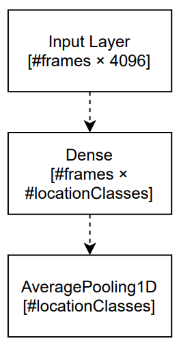
In this case, an Average Pooling layer’s forming sets size is 20 × 1. Using this size in average-pooling layer, we get again one number for each class, which returns a probability distribution over the set of scene locations.
Apart form average pooling, we have tried also max pooling. However, it led to substantially worse results. Its classification of the scene location was typically based on people or items in the foreground, not on the scene as a whole.
Although using the average-pooling layer is easy, it gives acceptable results. The number of trainable parameters of the network is then low, which makes it suitable for our comparatively small dataset.
3.2.4 Long Short Term Memory
An LSTM layer is used for classification of sequences of feature vectors, or equivalently, multidimensional time series with discrete time. Alternatively, that layer can be also employed to obtain sequences of such classifications, i.e., in situations when the neural network input is a sequence of feature vectors and its output is a a sequence of classes, in our case of scene locations. LSTM layers are intended for recurrent signal propagation, and differently to other commonly encountered layers, they consists not of simple neurons, but of units with their own inner structure. Several variants of such a structure have been proposed (e.g., [5, 8]), but all of them include at least the following four components:
• Memory cells can store values, aka cell states, for an arbitrary time. They have no activation function, thus their output is actually a biased linear combination of unit inputs and of the values coming through recurrent connections.
• Input gate controls the extent to which values from the previous unit within the layer or from the preceding layer influence the value stored in the memory cell. It has a sigmoidal activation function, which is applied to a biased linear combination of the input and recurrent connections, though its bias and synaptic weights are specific and in general different from the bias and synaptic weights of the memory cell.
• Forget gate controls the extent to which the memory cell state is suppressed. It again has a sigmoidal activation function, which is applied to a specific biased linear combination of input and recurrent connections.
• Output gate controls the extent to which the memory cell state influences the unit output. Also this gate has a sigmoidal activation function, which is applied to a specific biased linear combination of input and recurrent connections, and subsequently composed either directly with the cell state or with its sigmoidal transformation, using a different sigmoid than is used by the gates.
Hence using LSTM layers a more sophisticated approach compared to simple average pooling. A LSTM, layer can keep hidden state through time with information about previous frames.
Figure 7 shows that the input to an LSTM layer is a 2D matrix. Its rows are ordered by the time of frames from the input scene. Every input frame in the network is represented by one vector. The output from the LSTM layer is a vector of the same size as in previous approaches, which returns a probability distribution over the set of scene locations.
3.2.5 Bidirectional Long Short Term Memory
An LSTM, due to its hidden state, preserves information from inputs that has already passed through it. Unidirectional LSTM only preserves information from the past because the only inputs it has seen are from the past. A Bidirectional LSTM runs inputs in two ways, one from the past to the future and one from the future to the past. To this end, it combines two hidden states, one for each direction.
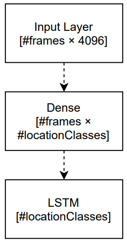
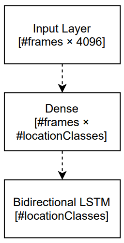
Figure 8 shows that the input to a bidirectional LSTM layer is the same as the input to a LSTM layer. Every input frame in the network is represented by one vector. The output from the Bidirectional LSTM layer is a vector of the same size as in previous approaches, which returns a probability distribution over the set of scene locations.
This paper is available on arxiv under CC0 1.0 DEED license.

