
Authors:
(1) Albert Gu, Machine Learning Department, Carnegie Mellon University with Equal contribution ([email protected]);
(2) Tri Dao, Department of Computer Science, Princeton University with Equal contribution ([email protected]).
Table of Links
3 Selective State Space Models and 3.1 Motivation: Selection as a Means of Compression
3.2 Improving SSMs with Selection
3.3 Efficient Implementation of Selective SSMs
3.4 A Simplifed SSM Architecture
3.5 Properties of Selection Mechanisms
4 Empirical Evaluation and 4.1 Synthetic Tasks
4.4 Audio Modeling and Generation
4.5 Speed and Memory Benchmarks
6 Conclusion, Acknowledgments and References
A Discussion: Selection Mechanism
B Related Work and B.1 S4 Variants and Derivatives
B.4 Linear Attention and B.5 Long Context Models
D Hardware-aware Algorithm For Selective SSMs
E Experimental Details and Additional Results and E.1 Synthetic Tasks
E.3 DNA Modeling
E.3.1 Pretraining Details
We describe the dataset and training procedure of the HG38 pretraining task in more detail.
E.3.2 Scaling: Model Size Details
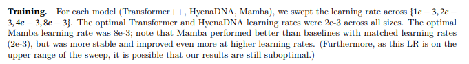
Models. The models we consider are:
• Transformer++: a Transformer with improved architecture, notably the usage of RoPE positional encodings (Su et al. 2021). Informally, we found these to be noticeably better than vanilla positional encodings from (Vaswani et al. 2017).
• HyenaDNA: the Hyena model from Nguyen, Poli, et al. (2023) and Poli et al. (2023), which is roughly a Transformer with the MHA block replaced by an H3 block using a global convolution parameterized by an MLP.
• Mamba: the standard Mamba architecture.
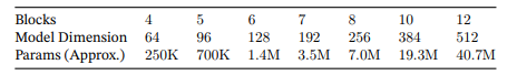
Model Sizes. We use the following model sizes.
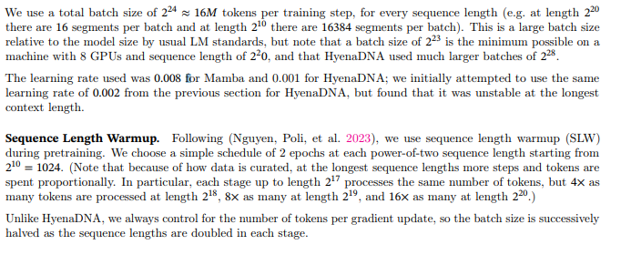
E.3.3 Scaling: Context Length Details
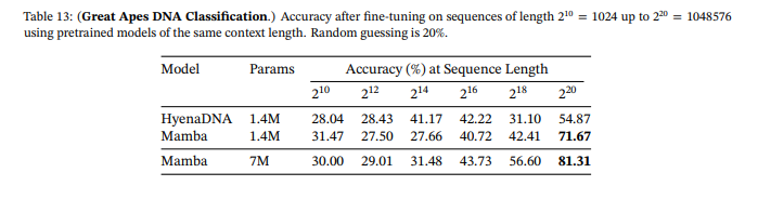
E.3.4 Species (Great Apes) Classi cation
Training consists of 10 epochs, each of which has 1024 gradient steps. Each gradient step uses batch size 64, which are all independently randomly drawn by uniformly picking a species, uniformly picking a chromosome, and then uniformly picking a contiguous segment of DNA.
Results for the Species classification task are in Table 13.
E.4 Audio Details
E.4.1 YouTubeMix Audio Pretraining
Model. We use a model with 3 blocks per stage (3 × 5 = 15 total Mamba blocks), pooling factor p = 16, and outer dimension D = 64, for about 3.5M parameters.
Dataset. The data is mu-law encoded at 8 bits, so the model is modeling discrete tokens with a vocab size of 256.
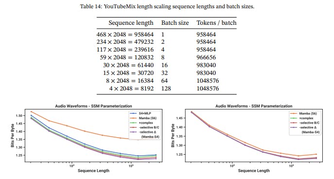
The dataset consists of clips of up to 1 minute long, or length 960000, which is subsampled and divided into segments of any desired sequence length. Since the architecture involves two stages of pooling by a factor of 16
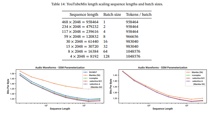
and we want the resulting sequence length to be a a multiple of 8 for hardware efficiency, the longest possible sequence is 468 × 2048 = 958464. The rest of our sequence lengths are defined by successively halving this and rounding up to the nearest multiple of 2048.
Table 14 lists the specifications used in Figure 7. Beyond the varying batch sizes, the number of valid segments in the training set varied between different sequence lengths (e.g. the number of training steps per epoch was not constant for different points in the graph), which may have contributed to kinks in the scaling curves.
Training. Models were trained for 200K training steps with a maximum learning rate of 0.002, 20K (10%) warmup steps, and weight decay 0.1 (similar to our general pretraining recipe across domains).
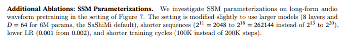
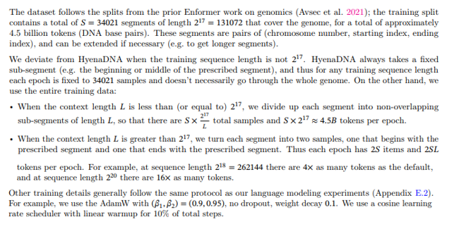
Figure 10 shows that the change from S4 → S6 (i.e. the selection mechanism) is not always beneficial. On long-form audio waveforms, it in fact significantly hampers performance, which may be intuitive from the point of view that audio is uniformly sampled and very smooth, and therefore benefits from continuous linear time-invariant (LTI) methods. After ablating away the selection mechanism, note that the resulting model is the S4 layer inside the Mamba block. To disambiguate, we call this Mamba-S4 as opposed the default Mamba architecture Mamba-S6.
However, on the right side, we keep the outer layers of the U-Net Mamba-S4 and ablate only the inner layers. The performance differences shrink dramatically; this reinforces the hypothesis that layers closer to the raw audio signal should be LTI, but once they are “tokenized” and compressed by the outer layers, the inner layers no longer need to be LTI. In this setting however, the real-valued SSM still underperforms the complex-valued one.
E.4.2 SC09 Speech Generation
Autoregressive training largely followed the autoregressive language modeling protocol, such as
We used a learning rate of 0.002 and 200000 training steps at a batch size of 16.
The large Mamba model in Table 4 has 15 layers per stage with an outer dimension of D = 96 and pooling factor 4. We note that this dataset is small (training went through 100 epochs) and for this large model, there was significant overfitting of the BPB or NLL. However, automated metrics of generated samples continually improving throughout training.
E.5 Efficiency Benchmark
Scan Operation. We compare the core operation of selective SSMs, which is the parallel scan (Section 3.3), against convolution and attention, measured on an A100 80GB PCIe GPU. Note that these do not include the cost of other operations outside of this core operation, such as computing the convolutional kernel in global-convolution models, or computing the QKV projections in attention.

Our scan implementation fuses the discretization step and the parallel scan, avoiding the cost of materializing all the large parameters in HBM.
For convolution, we use the standard implementation in PyTorch, which separately performs FFTs on the inputs and the filters, multiply them in frequency domain, then performs an inverse FFT to obtain the result. The theoretical complexity is O(L log(L)) for sequence length L.
For attention, we compare against the fastest implementation that we are aware of (FlashAttention-2 (Dao 2023)), with causal mask. Note that FlashAttention-2 with causal mask is about 1.7× faster than without causal mask, since approximately only half of the attention entries are computed.
End-to-end Inference. We measure the inference throughput of a Mamba 1.4B model and an untrained Mamba 6.9B model, against a standard Transformer (GPT3 architecture) at 1.3B and 6.7B size. We use the standard Transformer implementation in the Huggingface transformers library.
We set the prompt length to be 2048 and the generation length to be 128. We vary the batch size from 1, 2, 4, 8, 16, 32, 64, to 128, and measure time time taken to generate 128 tokens. We then calculate the throughput (tokens/s) as batch size × 128∕time taken. We repeat the measurements 3 times and take the average. Measurements are done on an A100 80GB PCIe GPU.
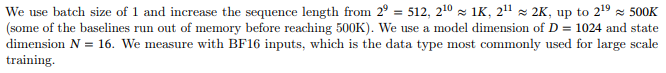
Memory Benchmark. The memory usage simply scales proportionally to the size of the activation tensors, as with most deep sequence models. We report measurements of the training memory requirements of 125M models
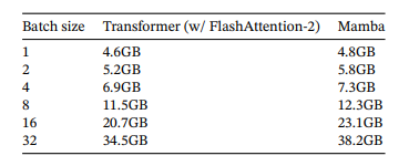
on 1 A100 80GB GPU. Each batch consists of sequences of length 2048. We compare to the most memory-efficient Transformer implementation we are aware of (with kernel fusion from torch.compile and with FlashAttention-2). Table 15 shows that Mamba’s memory requirement is comparable to a similar-sized Transformer with an extremely optimized implementation, and we expect further improvement in Mamba’s memory footprint in the future.
This paper is available on arxiv under CC BY 4.0 DEED license.